text processing – 67 Bricks developer blog

Things Customers Don’t Understand About Search

Note, this post is based on a dev forum put together by Chris.

Full-text search is a common feature of systems 67 Bricks build. We want to make it easy for users to find relevant information quickly often through a faceted search function. Understanding user needs and building a top notch user experience is vital. When building faceted search, we generally use either ElasticSearch (or AWS’s OpenSearch) or MarkLogic. Both databases offer very similar feature sets when it comes to search, though one is more targetted towards JSON based documents and the other, XML.

Search can seem magical at first glance and do some amazing things but this can lead to situations where customers (and UX/UI designers) assume the search mecahnism can do more than it can. We frequently find a disconnect between what is desired and what is feasable with search systems.

There are 2 main categories of problems we often see are:

Customers / Designers asking for things that could be done, but often come with nasty performance implications
Features that seem reasonable to ask for at first glance, but once dug into reveal logical problems that make developing the feature near impossible

Faceted Search

Faceted search systems are some of the most common systems we build at 67 Bricks. The user experience typicallly starts with a search box that they enter a number of terms into, hit enter and then be presented with a list of results in some kind of relevancy order. Often there is a count of results displayed alongside a pagination mechanism to iterate through the results (e.g. showing results 1-10 of 12,464). We also show facets, counts for how many results fit into different buckets. All this is handled in a single query that often takes less than 100ms which seems miraculous. Of course, this isn’t magic, full-text search systems use a variety of clever indexes to make searching and computing the facet counts quick.

Lets make a search system for a hypothetical website cottagesearch.com. Our first screen will present the user with some options to select a location, the date range they want to stay and how many guests are coming. We perform the search and show the matching results. How should we display the results and more importantly, how do we show the facets?

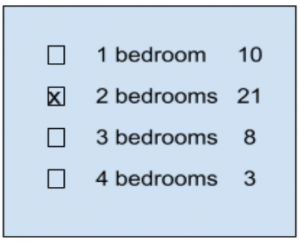
Let’s say we did a search for 2 bedroom cottages. We’ve seen wireframes for a number of occassions where the facet count for all bedroom numbers are displayed. So users see the number of results applicable to each bedroom count they would get if they didn’t limit the search to just 2 bedrooms (i.e. there aren’t that many 2 bed options, but look at how many 3 bed options are available). At first glance, this seems like a sensible design, but fundmanetally breaks how search systems work with faceting, they will return counts, but only for the search just done.

We could get around this by doing 2 searches, 1 limited by bedrooms and one that does not to retrieve the facet counts. This may seem like a sensible idea when we have 1 facet, but what do we do when we have more? Do we need to do multiple searches, effectively making an N+1 problem? How to we display numbers? Should the counts for the location facet include the limit of bedrooms or not? As soon as we start exploring additional situations we start to see the challenges the original design presents.

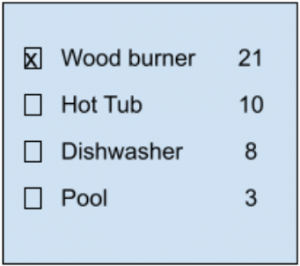
This gets harder when we consider non-exclusionary facets. Let’s say our cottage search system lets you filter by particular features, such as a wood burner, hot tub or dishwasher. Now, if we show counts of non-selected facets, what do these numbers represent? Do they include results that already include the selected facet or not? Here, the logic starts to break down and becomes ever more confusing to the end user and difficult to implement for the developer.

Other Complex Facet Situations

A common question we need to ask with non-exclusionary facets: Is it an AND or an OR search? The answer is very domain dependant, but either way we suggest steering away from facets counts in these situations.

Date ranges provide an interesting problem, some sites will purposefully search outside of the selected range so as to provide results near the selected date range. This may be a useful or annoying depending on what the user expects and is trying to achieve. Some users would want exact matches and would have no interest in results that do not meet the selected date range.

Ordering facets is also a questions that may be overlooked. Do you order lexographically or do you order by descending number of matches? What about names, year ranges or numeric values? Again, a lot of what users expect and would want comes down to the domain being dealt with and the needs of the users.

When users select a new facet, what should the UI do? Should the search immediately rerun and the results and facets update or should there be a manual refresh button the user has to select before the search is updated? An immediate refresh would be slower, but let users narrow down carefully, while a manual update would reduce the number of searches done, but then users may be able to select a number of facets in such a way that no results would be returned.

Hierarchies can also prove tricky. We often see taxonomies being used to inform facets, say subjects with sub categories. How should these be displayed? Again there are many solutions to pick from with different sets of trade-offs.

Advanced Search

Advanced search can often be a bit like a peacocks tail – something that looks impressive, but doesn’t contribute a fair share of value based on how much effort it takes to develop. A lot of designers and product owners love the idea of it but in practice, it can end up being somewhat confusing to use and many end users end up avoiding it.

Boolean builders exist in many systems where the designer of advanced search will insist on allowing users to build up some complex search with lots of boolean AND/OR options, but displaying this to users in a way they can understand is challenging. If a user builds a boolean search such as: GDP AND Argentina OR Brazil do we treat it as (GDP AND Argentina) OR Brazil or should it be interpreted as GDP AND (Argentina OR Brazil). We could include brackets in the builder, but this just further complicates the UI.

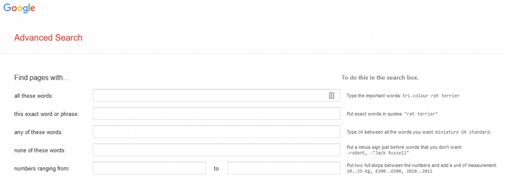
We frequently get bugs and feedback on advanced search, some of this feedback can amount to different users having contradictory opinions on how it should work. We would ask product owners to carefully consider “How many people will use it?” Google has a well build UI for advanced search that does away with the challenges of boolean logic by having separate fields for ANDs ORs and NOTs.

An advanced search facility can introduce additional complexity when combined with facets. If an advances search lets you select some facets before completing the search, does this form part of the string in the search box? We have had mixed results with enabling power users to enter facets into search fields (e.g. bedrooms:3), but this can be tricky, some users can deal with it, but others may prefer a advanced search builder while others will rely on facets post search.

Summary

In conclusion, we have 3 main takeaways

Search is much more complex than it first appears
Facets are not magic, just because you can draw a nice wireframe doesn’t make it feasable to develop
Advanced search can be tricky to get right and even then, only used by a minority of users

We’ve build many different types of search and have experimented with a number of approaches in the past and we offer some tried and tested principles:

Make searches stateless – Don’t add complexity by trying to maintain state between facets changes, simply treat each change as a fresh search. That way URLs can act as a method of persistence and bookmarking common searches.
Have facets only display counts for the current search and do not display counts for other facets once one has been selected within that category.
Only use relevancy as the default ordering mechanism – You may be tempted to allow results to be ordered in different ways, such as published date, but this can cause problems with weakly matching, but recent results appearing first.
Don’t build an advanced search unless you really need to and if you have to, use a Google style interface over a boolean query builder.
Check that search is working as expected – Have domain experts check that searches are returning sensible results and look into using analytics to see if users are having a happy journey through the application (i.e. run a search and then find the right result within the first few hits).
Beware of exhaustive search use cases – As many search mechanisms work on some score based on relevancy to the terms entered, having a search that guarantees a return of everything relevant can be tricky to define and to develop.

Dev Forum – Parsing Data

Last Friday we had a dev forum on parsing data that came up as some devs had pressing question on Regex. Dan provided us with a rather nice and detailed overview of different ways to parse data. Often we encounter situations where an input or a data file needs to be parsed so our code can make some sensible use of it.

After the presentation, we looked at some code using the parboiled library with Scala. A simple example of checking if a sequence of various types of brackets has matching open and closing ones in the correct positions was given. For example the sequence ({[<<>>]}) would be considered valid, while the sequence ((({(>>]) would be invalid.

First we define the set of classes that describes the parsed structure:

object BracketParser {

  sealed trait Brackets

  case class RoundBrackets(content: Brackets)
     extends Brackets

  case class SquareBrackets(content: Brackets)
     extends Brackets

  case class AngleBrackets(content: Brackets)
     extends Brackets

  case class CurlyBrackets(content: Brackets)
     extends Brackets

  case object Empty extends Brackets

}

Next, we define the matching rules that parboiled uses:

package com.sixtysevenbricks.examples.parboiled

import com.sixtysevenbricks.examples.parboiled.BracketParser._
import org.parboiled.scala._

class BracketParser extends Parser {

  /**
   * The input should consist of a bracketed expression
   * followed by the special "end of input" marker
   */
  def input: Rule1[Brackets] = rule {
    bracketedExpression ~ EOI
  }

  /**
   * A bracketed expression can be roundBrackets,
   * or squareBrackets, or... or the special empty 
   * expression (which occurs in the middle). Note that
   * because "empty" will always match, it must be listed
   * last
   */
  def bracketedExpression: Rule1[Brackets] = rule {
    roundBrackets | squareBrackets | 
    angleBrackets | curlyBrackets | empty
  }

  /**
   * The empty rule matches an EMPTY expression
   * (which will always succeed) and pushes the Empty
   * case object onto the stack
   */
  def empty: Rule1[Brackets] = rule {
    EMPTY ~> (_ => Empty)
  }

  /**
   * The roundBrackets rule matches a bracketed 
   * expression surrounded by parentheses. If it
   * succeeds, it pushes a RoundBrackets object 
   * onto the stack, containing the content inside
   * the brackets
   */
  def roundBrackets: Rule1[Brackets] = rule {
    "(" ~ bracketedExpression ~ ")" ~~>
         (content => RoundBrackets(content))
  }

  // Remaining matchers
  def squareBrackets: Rule1[Brackets] = rule {
    "[" ~ bracketedExpression ~ "]"  ~~>
        (content => SquareBrackets(content))
  }

  def angleBrackets: Rule1[Brackets] = rule {
    "<" ~ bracketedExpression ~ ">" ~~>
        (content => AngleBrackets(content))
  }

  def curlyBrackets: Rule1[Brackets] = rule {
    "{" ~ bracketedExpression ~ "}" ~~>
        (content => CurlyBrackets(content))
  }


  /**
   * The main entrypoint for parsing.
   * @param expression
   * @return
   */
  def parseExpression(expression: String):
    ParsingResult[Brackets] = {
    ReportingParseRunner(input).run(expression)
  }

}

While this example requires a lot more code to be written than a regex, parsers are more powerful and adaptable. Parboiled seems to be an excellent library with a rather nice syntax for defining them.

To summarize, regexes are very useful, but so are parsers. Start with a regex (or better yet, a pre-existing library that specifically parses your data structure) and if it gets too complex to deal with, consider writing a custom parser.

Case Genie or How to Find Unknown Unknowns

It was Paul Magrath, Head of Product Development and Online Content at ICLR, who first used the late Donald Rumsfeld’s phrase to describe the business case for what later became known as Case Genie.

The idea was simple. Lawyers needed to discover historical cases that might impact a case they were preparing. Frequently-cited cases would already be known to them: they’d be at the tips of their fingers, ready to type into their skeleton argument; cases known to every barrister specialising in the field they were arguing; cases that had been cited many times both by other cases and in text books; or cases that had recently changed how the law should be interpreted, and were therefore big news within a narrowly-focused legal community.

But there may be some cases that are relatively unknown that might make all the difference. Enter Case Genie.

This blog post presents a technical overview of Case Genie. How, exactly, is it possible to find “unknown unknowns”?

Word embeddings

Document embeddings are considered the state-of-the-art way of finding similarities between documents. But before document embeddings come word embeddings. A good way to start to think about word embeddings, is to think about words in a document. Let’s take Milton’s Areopagitica as an example. This single work is our corpus (the body of text we’re interested in). Let’s take a single sentence from Milton’s Areopagitica:

Many a man lives a burden to the Earth; but a good Book is the precious life-blood of a master spirit, embalmed and treasured up on purpose to a life beyond life.

Now, if we take each distinct word, we can give it a score based on how often it occurs in the text:

  many  — 1
  a     — 5
  man   — 1
  lives — 1
  …etc…

Now imagine graphing three of these words. I’m choosing three because this is easy to visualise, but rather than take the first three words in the sentence, let’s take the following:

  a         — 5
  life      — 3
  treasured — 1

Imagine these graphed across the x, y and z axes: ‘a’ has the value 5 on the x axis; ‘life’ has the value 3 on the y axis; and ‘treasured’ has the value 1 on the z axis. Further, imagine that for each value, there is an arrow from the origin to the point along each axis, so that we have 3 arrows of different lengths pointing in different directions. Now, in mathematics a value with a direction is called a vector, so we can say that each distinct word within a corpus can be represented as a vector; and within a document, a vector’s value is the number of occurrences of the word within that document.

Three dimensions aren’t too hard to visualise. Extrapolating, we can add further axes, which is much harder to visualise; as many axes as there are distinct words. Each distinct word in the corpus will therefore be represented by a vector.

Of course, that’s just one sentence and there are many in Areopagitica. The full vector space is defined by the number of unique words in the corpus, let’s suppose there are 2,000 in Areopagitica. Initially this will sound confusing, but the word embedding for a given word is made up of a value for every vector in the vector space, which is the same as saying a value for every word. For each distinct word, its word embedding will therefore comprise 1,999 zero values and one non-zero value — 1. If we order the distinct words alphabetically, we can represent an embedding as an implicitly ordered array of numbers. Therefore, for each word embedding, the non-zero value will be in a different place; ‘a’ would be:

  1 0 0 0 0 0 0 0 0 0 0 0 0 0 0 0 …

whereas ‘and’ would be:

  0 1 0 0 0 0 0 0 0 0 0 0 0 0 0 0 …

This is crazily sparse; the cleverness comes when using AI to use all that empty space more wisely.

Algorithms like word2vec and fastText (there are other algorithms, but these are the two we looked at for ICLR) provide a more compact representation of word embeddings. Whereas with Areopagitica, using the algorithm I described above, we would need 2,000 values (dimensions) for each word, word2vec and fastText can use a few hundred dimensions. You can download a 300-dimensional model from the fastText website trained on 2 million words from Wikipedia. Word embeddings actually use floating point numbers, so the word ‘a’ in the fastText model we trained for ICLR starts:

  -0.20005 -0.019533 -0.15494 -0.11114 0.074793 0.1194 -0.046101 …

The model for ICLR has 600 dimensions, so there are 600 numbers for each word embedding.

Exactly how word2vec and fastText create these word vectors is outside the scope of this blog post. Essentially, you start by training a model from the corpus, which you feed to the tool. The corpus and the training algorithms define relationships between words or character combinations. The corpus used to train the model therefore determines how the words’ relationships are actually represented in the model. If you train with a French corpus, you will get good results when calculating document embeddings for French text; but you would get bad results if you presented English text. In the same vein, if you train a model using legal documents, you will get a model that is more sensitive to legal meanings and definitions.

So, if we were to use Areopagitica as our corpus, we would have a model trained to recognise only uses of the words as used in Areopagitica. We could calculate sentence embeddings (which we could treat like document embeddings) for every sentence in Areopagitica to determine which sentences were most similar. However, the results would likely be quite poor. The reason for this is that the corpus is too small. Ideally, you need a lot of words, the more the better. For ICLR, we used all of the judgment transcripts and Case Reports contained in ICLR.online as our corpus. This represents around 200,000 documents; about 600,000,000 words.

But what are document embeddings, and how do you create them?

Document embeddings

Once you have word embeddings, you will want to create document embeddings. To create a document embedding, take all the word embeddings of the document and use cosine similarity to combine the dimensions into a single representation with the same number of dimensions.

Cosine similarity combines two vectors by calculating the cosine of the angle between them and multiplying by the length of the side not participating in the cosine calculation.

Cosine similarity is a nice way to explain it visually, but there is an algebraic isomorphism using dot products of normalised vectors.

This algorithm combines word embeddings into document embeddings:

Create an empty embedding (where all values are 0) called A. This is our aggregate.
For each word embedding, w:
1. normalise w;
2. for each value in A, add the corresponding value in w (add the first number in A to the first number in w, the second number in A to the second number in w, and so on).
Divide each value in A by the number of words used to calculate it.

To normalise a word embedding, take the square root of the sum of each value’s square (let’s call it n); then divide each value in the embedding by n.

This is the implementation used by fastText. However we have tweaked the algorithm to make use of tf–idf. tf–idf weights words that are considered important. A word is considered important if its frequency within the corpus is low compared to its frequency within a document. Since words like ‘a’ occur throughout the corpus, it is weighted low; whereas a word like ‘theft’ will be weighted higher, because it occurs only in a subset of documents within the corpus.

Calculating the distance between document embeddings

The final puzzle piece is to quantify how similar documents are based on their document embeddings. The distance between two documents is used as an indication of how similar they are. Documents that are close together are more similar than those that are further away.

To calculate the distance between two document embeddings, Cosine Similarity can be used again. This time, the vectors of the document embeddings are collapsed to a single value between 0 and 1. Identical documents have the value 1, completely orthogonal documents have the value 0.

We use a library called Faiss, created by Facebook Research, to store and query document embeddings. This is very fast, and you can query multiple input embeddings simultaneously.

And finally…

This post describes some of the major components used in Case Genie and delves a little into the concepts and some of the algorithms; but there is a lot more that I don’t have time to cover: specifically, how do we prepare the text of the corpus for training the model? I will cover that in another post.