It was Paul Magrath, Head of Product Development and Online Content at ICLR, who first used the late Donald Rumsfeld’s phrase to describe the business case for what later became known as Case Genie.
The idea was simple. Lawyers needed to discover historical cases that might impact a case they were preparing. Frequently-cited cases would already be known to them: they’d be at the tips of their fingers, ready to type into their skeleton argument; cases known to every barrister specialising in the field they were arguing; cases that had been cited many times both by other cases and in text books; or cases that had recently changed how the law should be interpreted, and were therefore big news within a narrowly-focused legal community.
But there may be some cases that are relatively unknown that might make all the difference. Enter Case Genie.
This blog post presents a technical overview of Case Genie. How, exactly, is it possible to find “unknown unknowns”?
Word embeddings
Document embeddings are considered the state-of-the-art way of finding similarities between documents. But before document embeddings come word embeddings. A good way to start to think about word embeddings, is to think about words in a document. Let’s take Milton’s Areopagitica as an example. This single work is our corpus (the body of text we’re interested in). Let’s take a single sentence from Milton’s Areopagitica:
Many a man lives a burden to the Earth; but a good Book is the precious life-blood of a master spirit, embalmed and treasured up on purpose to a life beyond life.
Now, if we take each distinct word, we can give it a score based on how often it occurs in the text:
  many  — 1
  a     — 5
  man   — 1
  lives — 1
  …etc…
Now imagine graphing three of these words. I’m choosing three because this is easy to visualise, but rather than take the first three words in the sentence, let’s take the following:
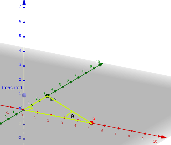
  a         — 5
  life      — 3
  treasured — 1
Imagine these graphed across the x, y and z axes: ‘a’ has the value 5 on the x axis; ‘life’ has the value 3 on the y axis; and ‘treasured’ has the value 1 on the z axis. Further, imagine that for each value, there is an arrow from the origin to the point along each axis, so that we have 3 arrows of different lengths pointing in different directions. Now, in mathematics a value with a direction is called a vector, so we can say that each distinct word within a corpus can be represented as a vector; and within a document, a vector’s value is the number of occurrences of the word within that document.

Three dimensions aren’t too hard to visualise. Extrapolating, we can add further axes, which is much harder to visualise; as many axes as there are distinct words. Each distinct word in the corpus will therefore be represented by a vector.
Of course, that’s just one sentence and there are many in Areopagitica. The full vector space is defined by the number of unique words in the corpus, let’s suppose there are 2,000 in Areopagitica. Initially this will sound confusing, but the word embedding for a given word is made up of a value for every vector in the vector space, which is the same as saying a value for every word. For each distinct word, its word embedding will therefore comprise 1,999 zero values and one non-zero value — 1. If we order the distinct words alphabetically, we can represent an embedding as an implicitly ordered array of numbers. Therefore, for each word embedding, the non-zero value will be in a different place; ‘a’ would be:
1 0 0 0 0 0 0 0 0 0 0 0 0 0 0 0 …
whereas ‘and’ would be:
0 1 0 0 0 0 0 0 0 0 0 0 0 0 0 0 …
This is crazily sparse; the cleverness comes when using AI to use all that empty space more wisely.
Algorithms like word2vec and fastText (there are other algorithms, but these are the two we looked at for ICLR) provide a more compact representation of word embeddings. Whereas with Areopagitica, using the algorithm I described above, we would need 2,000 values (dimensions) for each word, word2vec and fastText can use a few hundred dimensions. You can download a 300-dimensional model from the fastText website trained on 2 million words from Wikipedia. Word embeddings actually use floating point numbers, so the word ‘a’ in the fastText model we trained for ICLR starts:
-0.20005 -0.019533 -0.15494 -0.11114 0.074793 0.1194 -0.046101 …
The model for ICLR has 600 dimensions, so there are 600 numbers for each word embedding.
Exactly how word2vec and fastText create these word vectors is outside the scope of this blog post. Essentially, you start by training a model from the corpus, which you feed to the tool. The corpus and the training algorithms define relationships between words or character combinations. The corpus used to train the model therefore determines how the words’ relationships are actually represented in the model. If you train with a French corpus, you will get good results when calculating document embeddings for French text; but you would get bad results if you presented English text. In the same vein, if you train a model using legal documents, you will get a model that is more sensitive to legal meanings and definitions.
So, if we were to use Areopagitica as our corpus, we would have a model trained to recognise only uses of the words as used in Areopagitica. We could calculate sentence embeddings (which we could treat like document embeddings) for every sentence in Areopagitica to determine which sentences were most similar. However, the results would likely be quite poor. The reason for this is that the corpus is too small. Ideally, you need a lot of words, the more the better. For ICLR, we used all of the judgment transcripts and Case Reports contained in ICLR.online as our corpus. This represents around 200,000 documents; about 600,000,000 words.
But what are document embeddings, and how do you create them?
Document embeddings
Once you have word embeddings, you will want to create document embeddings. To create a document embedding, take all the word embeddings of the document and use cosine similarity to combine the dimensions into a single representation with the same number of dimensions.
Cosine similarity combines two vectors by calculating the cosine of the angle between them and multiplying by the length of the side not participating in the cosine calculation.
Cosine similarity is a nice way to explain it visually, but there is an algebraic isomorphism using dot products of normalised vectors.
This algorithm combines word embeddings into document embeddings:
- Create an empty embedding (where all values are 0) called A. This is our aggregate.
- For each word embedding, w:
- normalise w;
- for each value in A, add the corresponding value in w (add the first number in A to the first number in w, the second number in A to the second number in w, and so on).
- Divide each value in A by the number of words used to calculate it.
To normalise a word embedding, take the square root of the sum of each value’s square (let’s call it n); then divide each value in the embedding by n.
This is the implementation used by fastText. However we have tweaked the algorithm to make use of tf–idf. tf–idf weights words that are considered important. A word is considered important if its frequency within the corpus is low compared to its frequency within a document. Since words like ‘a’ occur throughout the corpus, it is weighted low; whereas a word like ‘theft’ will be weighted higher, because it occurs only in a subset of documents within the corpus.
Calculating the distance between document embeddings
The final puzzle piece is to quantify how similar documents are based on their document embeddings. The distance between two documents is used as an indication of how similar they are. Documents that are close together are more similar than those that are further away.
To calculate the distance between two document embeddings, Cosine Similarity can be used again. This time, the vectors of the document embeddings are collapsed to a single value between 0 and 1. Identical documents have the value 1, completely orthogonal documents have the value 0.
We use a library called Faiss, created by Facebook Research, to store and query document embeddings. This is very fast, and you can query multiple input embeddings simultaneously.
And finally…
This post describes some of the major components used in Case Genie and delves a little into the concepts and some of the algorithms; but there is a lot more that I don’t have time to cover: specifically, how do we prepare the text of the corpus for training the model? I will cover that in another post.